Generating samples: re-writing Bayes Rule as a probabilistic AI hack

Introducing the sayable through the visible

Demis Hassabis, co-founder of London-based, Google-owned DeepMind, speaks of the shift from hacker culture to a scientific culture at Google AI, the arm of Alphabet Corporation leading on ML/AI:

One reason we teamed up with Google back in 2014 was, Google …. came out of a research project that Larry and Sergey were doing at their PhDs, right? So I felt they were already very scientific, of all the big companies, in their approach, right? So it’s a very good match for how I was running DeepMind and how we run Google DeepMind — it’s scientific approach, scientific method. That’s the best method we’ve ever invented for understanding things in the world. Unbelievably powerful from the days of the Enlightenment, right? That’s what, quote, “created” the modern world and all the benefits of the modern world. So we got to double down on that method and trust that method. That would be my approach, versus alternative methods, which are very effective as well, but I think less correct for this type of technology, like a hacker-growth mentality, move fast and break things, you sometimes hear as the Valley mantra.¹

Hassabis, holder of a PhD in neuroscience, former chess prodigy and video game designer, co-recipient of the 2024 Nobel prize in chemistry,² has led DeepMind researchers in the application of image-based techniques to epistemic/expert scientific and cultural targets. Alphafold, AlphaGo, and various Atari game-playing AI are among the most well-known of what we might call DeepMind’s ‘hyper-epistemic performances.’ ‘Hyper’ in the sense of very excited, they all share a ‘focus’ on finding ways of re-doing knowing. They typically introduce something difficult to formulate as a proposition or statement (e.g. best move in a high-level game of Go, predicting the deeply folded structure of a protein, optimising energy demand in a hyper-scale data centre) as a problem of generating samples from probability distributions. Practically, a situation such as playing Go is approached as an immense collection of images (e.g. images of the position of every piece at each move in many games of Go), and the model’s work is to generate an optimised proposition (e.g. best next move in the game) based on the image-aggregate.³ In the hyper-epistemics of ML/AI, the visible often conditions, we might say, the sayable, and sometimes, the sayable conditions the visible.

This rather strange yet not entirely novel way of introducing of what can be seen and what can be said to each other is a hallmark of a recent ML/AI shift in computation towards generative models.⁴ In the emerging ‘scientific approach’ of hyper-epistemic platforms, evidence, experiment, inference and prediction replace hacking and the putatively hacker culture of Silicon Valley as espoused, for instance, by the inhabitants of 1 Hacker Way, Meta Platform Inc. Hassabis rather unfortunately deflects attention away from this invention by both invoking (a) a classical image of modern science: ‘trust that method’; and (b) tendentiously identifying hacking with ‘platform growth mentality.’

It might be interesting and important to construct alternative readings of what is going on in ‘doubling down on method’, a scene in which systems of visibility centred on imaging join with systems for production of statements and propositions in a new formation. In his account of Michel Foucault’s Archaeology of Knowledge, Gilles Deleuze cuts to the basic issue:

each historical formation sees and reveals all it can within the conditions laid down for visibility, just as it says all it can within the conditions relating to statements.⁵

What contemporary computational cultures can see and what they can say, and how their seeing and saying join, together define an historical formation. The conditions of visibility and the conditions of sayability are not given but made together, yet without ever coinciding or converging. The recalcitrant divergence of saying and seeing, the sayable and the visible, and in Bayesian terms, the unobservables and the observables, is a, perhaps the, site of invention, thought and other things like that.

p(hack): Bayes Rule as a protocol for probability hacking

If any of this unstable, ongoing and elusive reconfiguration of saying and seeing is to be become accessible or thinkable, how would that happen? From Christopher Kelty, and contra Hassabis, I borrow the idea of the hack as a way of inhabiting computational structures. As Kelty puts it, ‘hacks can … be purely aesthetic or purely criminal: it is not the politics that makes the figure of the hacker useful, but the way it inhabits and observes existing structures, looking for concrete, technical ways to change them from the inside.’⁶ Hacks are often seen as quick fixes, but they can also embody deeper, more sustained engagements with computational structures. A hack bears within it a surprising, sometimes mischievous, profound, criminal, aesthetic, technical, or political relation to the structures it inhabits. A hack, like the one proposed in this paper, might be technically and scientifically wrong or ‘hairy’, but it does seek to inhabit rather than survey or randomly walk by at a distance.

The ‘existing structures’ in the scope of discussion here are joint probability distributions. In terms of classical probability theory, a joint probability distribution is perhaps the most comprehensive framing statistical framing of a given situation. It puts two or many variables in relation. It describes a whole system as function that assigns probabilities to every state of the system as defined by a combination of variables. The preliminary hacker problem is how to inhabit a joint probability distributions. And having taken up that position, the next problem is to identifying what a probability hack might look like. I envisage a probability hack, a p(hack), as a form of re-writing or re-diagramming the conditions under which samples are generated from joint probability distributions.

That said, joint probability distributions are difficult to work with: both analytically and synthetically. The shift to sampling as a way of approximating probability distributions that would otherwise, at least in classical conceptions of modern science, be attempted through application of mathematical analysis is a significant and perhaps momentous epistemic re-articulation. Most statistical models first reduce complexity by constructing approximations to joint probability distribution. For example, the many latent spaces of large language models approximate the joint probability distribution of the intricately nuanced sayable, and sampling from the latent space is the way to generate new utterances.

Bayes Rule offers especially flexible probability hacking scope. The elements of this simple probability theorem, the Bayes rule, delineate or diagram, to use Deleuze’s term, many practices of working on joint probability distributions. Bayes Rule-oriented computational devices such as Gibbs samplers (originally developed for the ‘Bayesian restoration’ of degraded images),⁷ the Metropolis-Hastings algorithm⁸ (both variants of Markov Chain Monte Carlo methods),⁹ and hierarchical models more generally, are not generally used in ML/AI, but usefully focus attention on the practices of working with joint probability distributions. On the scene of the Bayes Rules probability hack, some of the features to be observed include computational renderings of joint probability distributions, modes of sample generation from joint probability distributions, and practices of repeated updating in order to approximate.

It will be necessary to re-write the theorem in different ways to disentangle changes associated with sample generation. As a point of reference, I draw on a highly cited, multi-edition textbook of Bayesian statistics, Bayesian Data Analysis.¹⁰ Other useful sources include programming guides for ‘Bayesian hacking.’¹¹ At times, it helps to prompt various generative models to assist in re-writing the theorem as simulations. (Those generative models are themselves joint probability distributions). Finally I ground the computational structures in technical fragments, events, announcements, and devices found on the scene of contemporary sampling practices. Most of these are quite well-known already, but I endeavour to re-orient them around the saying/seeing nexus and re-configuration through sample generation.

The experimental method for a probability hack — hereafter referred to as p(hack) — is then be an imitative re-writing process:

1. present the Bayes Rule joint probability theorem, re-writing it slightly as a diagram of computational processes;
2. read a high-cited Bayesian statistics textbook with an eye for how different elements of the diagram of computational processes are held together;
3. generate code-based simulations for any piece of that process that seems especially difficult, significant or open-ended;
4. connect and align elements of the simulations and diagram with concrete pieces, utterances, fragments and elements found at that scene of computational culture.

Re-writing a statistical statement: the confluence

There is something quite diffuse going on in the reorganisation of images, words, devices, code and platforms through machine learning and AI. From the perspective of the p(hack), the decisive rupture associated with the contemporary computational turn to ML/AI is not the GPU, the transformer model, reinforcement learning,embeddings, multi-head attention or any other specific technique, but the rumble of many avalanches of probability distributions joining together. In various streams of action, but particularly along the fracture zones of images and texts (documents, labels, tags, captions, etc.), joint probability distributions are being generated, sampled, and approximated. The joint probability distribution is a computational seeing-saying, a seeing-saying join that is not reducible to either.

A single formulation, one that can be regarded as a fully-weighted ‘statement’ in the Foucauldian, archaeological sense of that term,¹² captures something of this confluence. The formulation is Bayes Rule (BR) as devised in the late 18th century by Reverend Thomas Bayes, and as re-formulated and re-written in the form of software and probabilistic programming languages in the late 20th century by statisticians and computer scientists:

p($\theta$\|y) = p($\theta$)p(y\|$\theta$)/p(y)

This formula is drawn from Gelman, Carlin, Stan and Rubin’s widely-cited, multi-edition textbook ``{=html}Bayesian Data Analysis``{=html}.¹³

Very many shall we say ‘theorematic’ explanations of BR are available and readers might benefit from reading some of them (e.g. “Bayes’ Rule is a fundamental concept in probability theory that describes how to update the probability of a hypothesis when given new evidence. Let me break it down systematically … The beauty of Bayes’ Rule is how it mathematically formalizes the process of learning and updating our understanding based on new evidence.” Anthropic Claude AI; https://claude.ai/chat/e4b3e159-f213-457e-be53-63c5842c64b2).

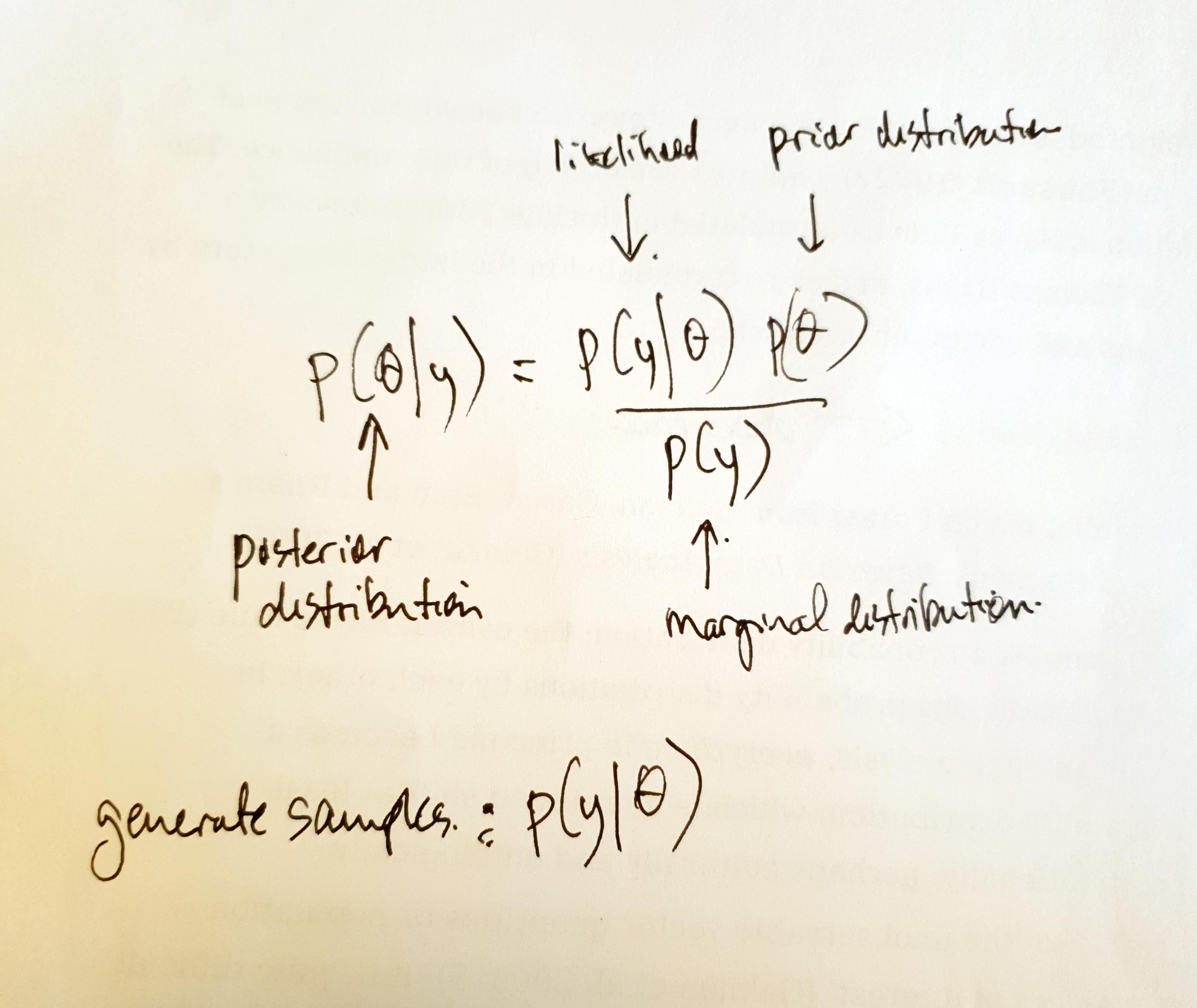
A p(hack)-motivated account differs from these in its attention to the techniques, infrastructures and computational arrangements associated with. Thus, in this rendering/sampling of BR:

• p(..) denotes a probability distribution; the overall Bayes Rule
  multiplies/divides probability distributions by each other; in
  Bayesian data analysis, ``{=html}everything``{=html} becomes
  a probability distribution in principle which is a profound shift at
  least computationally, and perhaps culturally and ontologically;
• $\theta$ refers to ‘the unobservable vector quantities or population
  parameters of interest’;¹⁴ it is difficult to overstate current
  interest and investment in $\theta$s for approximating $\theta$s
  supports prediction; BR provides a way to estimate $\theta$; that is
  why $p(\$theta)$ lies on the left-hand side of the expression, the
  side of the expression that holds the results;
• y is ‘the observed data’;¹⁵ the slender inscription of the data,
  all observation, anything sensed, measured or extracted from an
  archive in the single poignant ‘y’ barely hints at its somewhat
  voluminous character in the silos strewn across the sciences,
  industries, media, institutions and governments today; also note that
  y, as contrasted with x, is usually the symbol for what is predicted
  or inferred, so in this ambiguous usage, it is both what is observed
  and what could be observed; a generated sample, for instance, is still
  a y;\
• the vertical bar \|, which occurs twice, means ‘conditioned on’, or
  ‘given that’; so the left-hand side of the formula can be read as the
  probability of $\theta$ given the values of y; despite appearances,
  this bar is not solid; it is riddled with criss-crossings; this
  slender stroke writhes with complications;\
• overall, viewed as a piece of arithmetic, the right-hand side of the
  formula is a ratio of two products: the numerator is the product or
  multiplication of the prior distribution of $\theta$ and the
  ‘likelihood’ of the data given what is already known of $\theta$; the
  denominator is the ‘marginal distribution’ of the data, p(y); the
  terminological nuances on this front are less important than the
  general pattern of multiplying and dividing.

These few elements of the formula overlay a complex warren of computational practices. The ways in which probability can be distributed, for instance, vary widely, well-beyond the two dozen or so ‘standard,’ properly-named probability distributions (Poisson, Gaussian, Beta, Dirichlet, etc.). The actual mixing/multiplying of data (y) and theory/beliefs ($\theta$) in BR deeply erodes the neatly-edged and polished symbolic, deductive expressions of probability theory.

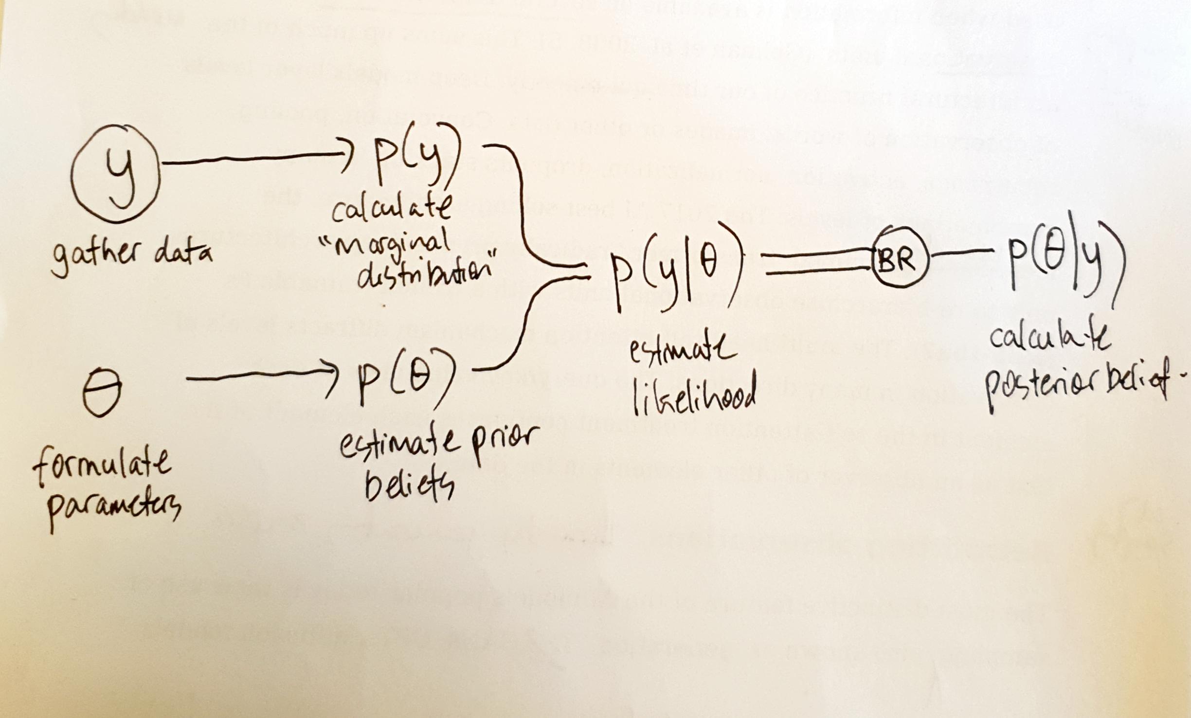
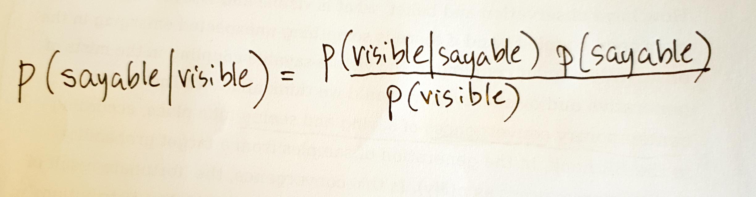
Is it good to speak in hacked statistical terms, saying for instance that contemporary computational culture is p(visible\|sayable)? The p(hack) is a way of using BR formula to account for a significant shift in computational practices. This re-writing literally sets up a ‘full probability models,’¹⁶ or more specifically, ‘a joint probability distribution for all observable and unobservable quantities’, then ‘conditioning on observed data’ and ‘evaluating the fit of the model’ over and over, and then, soon or later, generating samples a.k.a predictions from the model.

We encounter joint distributions of observable and unobservable, of y and $\theta$, of visibility and sayability in the millions of propositions put out by the large model endpoints at Microsoft, Google, Amazon, Alibaba, OpenAI, Anthropic, Meta Platforms, or any of their burgeoning contenders (DeepSeek, Grok3 from XAI, etc.). Their joint probability distributions have specific ontological or world-making effects, effects that are not limited to naming, identifying or segmenting the world.

We also know that, whether in the \$USD billions that platforms pour into data centre builds under the mounting pressure of AI loads, the drastic re-zoning of chip layout and architectures across the processor ecologies to include the many-core parallel computer epitomised by Nvidia GPUs, or the look-and-feel of stable-diffusion model-generated images suffusing the images/video-sharing platforms, sampling from joint probability distributions is highly invested. We might think too of effort going into transparency, accountability, alignment, interpretability of AI models. Signs of the problematisation of the joint probability distribution are everywhere, but difficult to read.

Sampling as a probability hack

The pivotal feature of Bayesian data analysis as detailed in the four hundred or so pages of Gelman et. al is sampling:

Fortunately, a battery of powerful methods has been developed over the past few decades for approximating and simulating from probability distributions.¹⁷

Many of the techniques used in ML/AI vary or expand the workflows of Bayesian computation: (1) posit initial or ``{=html}prior``{=html} beliefs as a combination of $\theta$; (2) work out p(y\|$\theta$) or the likelihood of observing y given those prior beliefs; (3) adjust the prior beliefs in a way that improves that likelihood; the ways of adjusting the prior beliefs vary but all hinge on some version of a random walk testing at each step if that likelihood improves; (4) repeat steps 2-3 until values of $\theta$ stabilise in a ‘stationary distribution.’ These computed $\theta$s, known as ‘posteriors,’ are then used to generate samples, predictions, or inferences.

(1) Sampling as approximation

BR is a grand unifying probability statement in its own right. Certain strands of Bayesian theory treat BR as greatly significant for science, knowledge and subjectivity more generally. For instance, there is a burgeoning Bayesian brain literature).¹⁸ But for the purpose of p(hacking), certain computational re-writings of BR are more important. In what is sometimes loosely called ‘simulation,’ Bayesian computation generates samples from a probability distribution ‘even when the density function cannot be explicitly integrated.’¹⁹

Sampling from a probability distribution — using a Gibbs sampler, or Markov Chain Monte Carlo algorithms such as Metropolis-Hastings, or the WinBUGs package — is a way of approximating something that cannot be calculated using the propositions and operations of mathematical analysis (e.g. differential or integral calculus).

[Animate 1: Gibbs sampler for the joint probability distribution of 2 normal/Gaussian distributions. The sampler generates samples from the joint distribution by repeatedly sampling from each of the two normal distributions, aloways using the sample value of the other distribution as a condition](https://claude.site/artifacts/c6d7f7c3-70a1-4c88-b17a-e5cf1214ed2a)

Anything that could have a number assigned to it, including any parameter, ‘constant’ or other form of value, become slightly less stable and definite since it could now appear as a probability distribution approximated via the repeated sampling done by, for instance, the Gibbs sampler in Animate 1. In Animate 1, the Gibbs sampler generates samples from the joint probability distribution of two normal/Gaussian distributions. The Animates used here are themselves samples from a joint probability distribution of the sayable and the visible, since the code that renders the animation (including the interface devices) comes from an LLM.

In other words, the shift that began in the mid-1970s, when Bayesian data analysis forswore ‘closed-form’ analytical solutions for the sake of generating samples by computation, altered the ground on which hitherto unobservable quantities such as population parameters stood.²⁰

[Animate 2: Metropolis-Hastings algorithm sampler for the joint probability distribution of 2 normal/Gaussian distributions. The sampler generates samples from the the joint distribution by repeatedly proposing samples and keeping only those with higher probabilites than the current state.](https://claude.site/artifacts/5abd3824-cc80-4113-a43d-5e79aeaacfa2)

Gainsaying exact or closed-form solutions, the computational enactments of BR approximate everything using some elegant hacks. The important class of Markov Chain Monte Carlo (MCMC) algorithms combine two approaches to probability (as seen in Animate 2). It combines the convergence properties of a random-walker sampling at every step the elevation of the terrain (Markov Chain) and always stepping uphill, and use of many random walkers starting from different positions (Monte Carlo method) to generate samples that spread out unevenly as a probability distribution. The computational apparatus of MCMC — the most powerful, widespread joint probability distribution modelling technique used in Bayesian analysis — hinges on a basic form of convergence called ‘stationarity.’ The thousands of steps taken by a team of random walkers all walking uphill eventually converge. While some get stuck on minor peaks, many will gather on the highest point.

Under the aegis of BR, everything unknown or unobservable takes the form of a computable probability distribution or a $\theta$, and the model is a joint probability distribution that specifies the probability of each and every combination of observable and unobservable.

(2) Sampling in the diffracted light of \|

Does BR – a way of approximating joint probability distributions by piling up samples — provide any traction in the avalanching series of revolutions currently experienced around both what can be said and what can be seen? The BR hack subjects the unobservable or sayable $\theta$ and the observable or visible $y$ to approximation, approximation not just as single point values but as a spectrum of values in the form of a probability distribution.

There is one central piece in the formula holding up the whole edifice of unobservables and observables: the vertical bar \| or ‘conditioned on.’ ‘Conditioning on observed data’ is the second step in Bayesian inference, and the one that attracts most of the ‘computational methodology,’²¹ as Gelman et. al. blithely observe. The \| can be found twice in the BR formula, once on the left of the expression and once on the right. The flipped re-writing of p($\theta$\|y) and p(y\|$\theta$) is axial. Through the vertical bars, observables and unobservables affect each other, and affect each many times over in the ‘update beliefs in the light of observation’ cycle that is the core workflow of the BR hack.

In the course of generating many samples to aid in approximating unobservables, $\theta$s are repeatedly conditioned by observations, and observations are conditioned by $\theta$s. Priors repeatedly become posteriors, blurring the classic epistemic divide of ``{=html}a priori``{=html} and ``{=html}a posteriori``{=html} found in Euclid,²² Kant²³ and much analytic philosophy.

(3) Sampling from many observables

The slender vertical bar also supports the composition of hierarchical architectures centred on probability distributions, whether it is the many layers of the now classic deep learning networks such as Resnet or VGG16,²⁴ the stages of multi-head attention in a transformer model, or the de-noising U-net in a diffusion model.²⁵ They are all arranged around $\theta$s numbering in the billions that they condition on y, the billions observables of this world.

The fact that nearly all diagrams of the present-day p($\theta$\|y) found in ML/AI have a hierarchical aspect is no accident when viewed in the diffracted light of ‘\|’. The conditioning vertical bar readily supports such architectures. As a result, the architecture of $\theta$ becomes long and labyrinthine, within many subtle conditionings of unobservables by other unobservables. The sprawling opacity of latent space in deep learning and other modelling practices takes root here. Hierarchical unobservables constructed from layered \| draw out from the often dreamy recesses of latent space certain hieratic AI-figures in the sacred Silicon Valley vestments of t-shirt-and-jeans uttering p(doom)s for their platforms.

Perhaps more importantly, ‘hierarchical models,’ Gelman et. al. write, ‘ … are used when information is available on several different levels of observational units’.²⁶ This sums up much of the architectural conditions under which joint probability distributions generate samples. Deep learning models weave partial observation of words, images or other data. Convolution, pooling, recurrence, activation, normalization, dropouts²⁷ stack up in many combinations of levels. At times, hierarchies collapse again. 2017’s best-selling AI architecture, the blandly-named ‘transformer,’ radically prunes deep architectures, only to re-hierarchise observational units with a trillion trainable $\theta$s.²⁸ The multi-head self-attention mechanism diffracts levels of observation in many directions. The query/key/value view of each element in the self-attention treatment configures each element of the text as an observer of other elements in the data.

(4) Sampling new observables

The most distinctive feature of the AI models popular today is a generalisation of sampling to generate text, audio, speech, images, code or other inscriptions. GANs, GPTs, diffusion models, and the like all generate samples from joint distributions of unobservable quantities conditioned by observations. On the one hand, despite being very large models (billions of parameters, etc.), none of them aim to model a full joint probability distribution (that is, to map the probability of every possible combination of the values of all the parameters; usually more combinations than atoms in the universe). In each case, there is some localization of the joint probability distribution through masking, a context window, or some such device. On other hand, viewed in aggregate, the many slight variations, combinations and permutations of generative models could be seen as an approximation to the full joint probability distribution of, say, the social field. This generalised sampling perhaps goes beyond BR practices. ‘Generation’ is undoubtedly still a quintessentially Bayesian approach to computation. At core the BR hack computes samples from a target distribution in order to update statements of $\theta$. Once $\theta$s or prior beliefs have been updated, predictions or inferences of $y$ follow. The twist in the generative ML/AI is the turn to sampling $y$ from the joint distribution of all unobservable quantities conditioned by observation: p($\theta$\|y) is used to drive p(y\|$\theta$).

An extended version of the BR workflow for sample generation runs through the training regimes of ML/AI: forwards pass -\> loss-calculation -\> back-propagation -\> update weights -\> repeat until convergence/optimisation -\> generate new observables (conditioned by prompts). Many of the specific techniques using during ML/AI training phases — regularization (constraining parameters within a limited range), dropouts (randomly removing connections), or early stopping (prior to final convergence), layer normalization (rescaling all $y$ values within a standard normal distribution) — can be considered in the light of BR as practices of updating unobservables encoded in the hierarchical architecture.

Beliefs in the world

This paper has suggested that Bayes Rule provides a diagrammatic device that maps the avalanching of probabilities through recent ML/AI systems such as convolutional, recursive, generative-adversarial, diffusion and transformer models.

Provisos applies to the use of the BR hack: BR should be read computationally rather than as a closed-world probability theorem. More specifically, BR should be re-written in the light of:

• (i) the re-binding of observables/unobservable in joint probability distributions;
• (ii) intricate hierarchical structures of conditioning;
• (iii) generating of sayable and visible via sampling;
• (iv) hyper-epistemic generalisation of sampling.

A minimal p(hack) of the contemporary computational nexus might be: sample the visible from the joint probability distribution of the sayable, and vice versa.

That hack might be too hirsute (a hacker term for overly complex hacking), but it posits a lively computational nexus of seeing and saying. The nexus of saying and seeing knits itself as the taciturn and blinkered machinery of probability distributions is mobilized outside the expert scientific knowledge settings, such as those described in Gelman’s ``{=html}Bayesian Data Analysis``{=html}, where it first emerged.

Whatever way we want to talk about AI & ML today is going to be conditioned by a diagrammatics of power rooted in sampling from joint probability distributions.The re-configurable form of BR (p($\theta$\|y) = p($\theta$)p(y\|$\theta$)/p(y)) or its re-writing as p(visible\|sayable) traces what Deleuze strikingly termed the ‘statistical curve’ of contemporary culture. It is a diagram of power, ‘linking, aligning and homogenizing particular features, placing them in a series and making them converge,’ as Deleuze puts it.²⁹ Integration of ‘the statistical curve’ — for this we might substitute ‘joint probability distribution’ — stabilises power relations via a multiplicity of points, engendering powers to affect and be affected in many aspects. As a result, new epistemic, affective and ontological gradients arise in the invertible sampling from p(sayable\|visible) and p(visible\|sayable).

Seeing $Y$ and saying ($\theta$) entwine in the BR hack. Caught up with each other in the joint probability distribution, how they affect each other across the vertical bar \| is always still a question of specific condition(ing)s of visibility and statements. More and more contextual $\theta$ flow into the models. We might think of how a generative image model such as Stable Diffusion³⁰ aligns the generation of image samples using text prompts. During training, the ‘cross-attention’ mechanism literally multiplies text embeddings (a.k.a $\theta$, themselves a product of a transformer large language model such as BERT or WordPiece),³¹ by image embeddings (a.k.a $\theta$), in shaping the generated sample images. Similarly, each ‘breakthrough’ — bi-directional encoding, multi-head attention, de-noising diffusion, etc. — conditions the joint probability distribution on some new combination of observable and unobservable quantities.

The segmentation and supple articulation through convergence-based sampling diffuse and propagate widely and quickly across institutions, sciences, industries and media because it re-introduces saying and seeing to each other.

The motivation to hack probability is twofold. Large-language models such as GPT-3 or BERT have been called ‘stochastic parrots.’³² Their social and existential ills have been attributed in part to a pervasive unwillingness to see them as statistical artifices that ‘parrot’/sample their own data. The charge that the ML/AI is ‘just statistics’ is problematic on several fronts. It assumes that we know what statistics is, and that statistics itself doesn’t change. The ‘no real knowledge’ complaint about joint probability models also predicates knowledge on an intentionality anchored in a privileged subject position. That predication has been tenuous and unstable for a long time on both practical and theoretical grounds. The increasingly effective and expansive multiplication of probability distributions in the BR hack makes it more obvious that there is nothing ‘behind’ even the most knowing practices. Good to be done with that privileging of human sapience.

What is perhaps most strikingly dissonant in most renderings of ML/AI-based computation is the hollowing out of joint probability distributions and their significance in generating samples. The p(hack) diverges from this position by questioning both the absence of (human) intentionality and the limits of computability in the dense terrain of joint probability distributions.

How come, if p($\theta$\|y) is so significant, sampling from joint probability distributions are not much more in view? Bayesian statistics is often sketched as ‘updating beliefs in the light of observation.’ The BR hack expands the scope of belief as such, and perhaps updates it in the light of the re-jointing of saying and seeing in p(sayable\|visible). Updating beliefs in the light of samples generated from joint probability distribution re-distributes belief in the world. In what might seem to be a highly untenable proposition, the simulations, the generation of samples from joint probability distributions, and the conditioning of saying and seeing on each other might practically have the effect of putting beliefs in the world. The question is: can we tolerate probabilities becoming animate in the world rather than risk-focused expressions of uncertainty or degrees of confidence?

References

Bender, Emily M., Timnit Gebru, Angelina McMillan-Major, and Shmargaret Shmitchell. “On the Dangers of Stochastic Parrots: Can Language Models Be Too Big? 🦜” In Proceedings of the 2021 ACM Conference on Fairness, Accountability, and Transparency, 610–23. FAccT ’21. New York, NY, USA: Association for Computing Machinery, 2021. doi: 10.1145/3442188.3445922.

Brooks, Stephen P. “Bayesian Computation: A Statistical Revolution.” Philosophical Transactions: Mathematical, Physical and Engineering Sciences 361, no. 1813 (2003): 2681–97. https://www.jstor.org/stable/3559268.

Davidson-Pilon, Cameron. Bayesian Methods for Hackers: Probabilistic Programming and Bayesian Inference. 1st edition. Addison-Wesley Professional, 2015.

Deleuze, Gilles. Foucault. First Edition. Minneapolis: University of Minnesota Press, 1988.

Devlin, Jacob, Ming-Wei Chang, Kenton Lee, and Kristina Toutanova. “BERT: Pre-training of Deep Bidirectional Transformers for Language Understanding.” In Proceedings of the 2019 Conference of the North, 4171–86. Minneapolis, Minnesota: Association for Computational Linguistics, 2019. doi: 10.18653/v1/N19-1423.

Euclid. The Thirteen Books of the Elements, Vol. 1. 2nd ed. edition. Dover Publications, 2012.

Foucault, Michel. Archaeology of Knowledge. London & New York: Routledge, 2013.

Gal, Yarin, and Zoubin Ghahramani. “Dropout as a Bayesian Approximation: Representing Model Uncertainty in Deep Learning.” In International Conference on Machine Learning, 1050–59. PMLR, 2016.

Gelman, Andrew, John B. Carlin, Hal S. Stern, and Donald B. Rubin. Bayesian Data Analysis. 2nd ed. Chapman and Hall/CRC, 2008.

Geman, S., and D. Geman. “Stochastic Relaxation, Gibbs Distributions, and the Bayesian Restoration of Images.” Pattern Analysis and Machine Intelligence, IEEE Transactions on, no. 6 (1984): 721–41.

He, Kaiming, Xiangyu Zhang, Shaoqing Ren, and Jian Sun. “Identity Mappings in Deep Residual Networks.” In European Conference on Computer Vision, 630–45. Springer, 2016.

Kant, Immanuel. Critique of Pure Reason. Translated by Norman Kemp-Smith. 2nd ed. Houndmill: Macmillan Publishers, 1963.

Kelty, Christopher. “Hacking the Social.” In Inventing the Social, edited by Noortje Marres, Michael Guggenheim, and Alex Wilkie. Mattering Press, 2018. doi: 10.28938/9780995527768.

Mackenzie, Adrian. Machine Learners: Archaeology of a Data Practice. Cambridge, MA: MIT Press, 2017.

Mackenzie, Adrian, and Anna Munster. “Platform Seeing: Image Ensembles and Their Invisualities.” Theory, Culture & Society, June 2019, 0263276419847508. doi: 10.1177/0263276419847508.

Metropolis, N., A. W. Rosenbluth, M. N. Rosenbluth, A. H. Teller, and E. Teller. “Equation of State Calculations by Fast Computing Machines.” The Journal of Chemical Physics 21 (1953): 1087.

Nobel. “The Nobel Prize in Chemistry 2024.” NobelPrize.org. https://www.nobelprize.org/prizes/chemistry/2024/hassabis/facts/, 2024.

Rombach, Robin, Andreas Blattmann, Dominik Lorenz, Patrick Esser, and Björn Ommer. “High-Resolution Image Synthesis with Latent Diffusion Models.” arXiv, April 2022. doi: 10.48550/arXiv.2112.10752.

Roose, Kevin, Casey Newton, Davis Land, Rachel Cohn, Jen Poyant, Chris Wood, Dan Powell, Marion Lozano, and Pat McCusker. “Google DeepMind C.E.O. Demis Hassabis on the Path From Chatbots to A.G.I.” The New York Times, February 2024.

Suess, Eric A., and Bruce E. Trumbo. Introduction to Probability Simulation and Gibbs Sampling with R. 1st Edition. New York: Springer, 2010.

Vaswani, Ashish, Noam Shazeer, Niki Parmar, Jakob Uszkoreit, Llion Jones, Aidan N. Gomez, Lukasz Kaiser, and Illia Polosukhin. “Attention Is All You Need.” arXiv, December 2017. doi: 10.48550/arXiv.1706.03762.

Yon, Daniel, and Chris D. Frith. “Precision and the Bayesian Brain.” Current Biology 31, no. 17 (2021): R1026–32.

Notes